Introduction:

A statistical framework called Bayesian Hierarchical Modeling allows Bayesian analysis to be applied to models that have nested structures. Because there are several levels of parameters in this model, each of which is modeled as a random variable, the model is hierarchical. It enables the modeling of intricate relationships between variables and the inclusion of previous data.

Concepts related to the topic:

Bayesian Modeling:

A method of statistical modeling that updates parameter beliefs in response to new data by applying Bayesian probability.

Bayesian Statistics:

A subfield of statistics known as "Bayesian Statistics" is concerned with updating a hypothesis's probabilities in response to new data or evidence. It bears Thomas Bayes' name, who applied what is now known as Bayesian inference to provide the first mathematical treatment of a non-trivial statistical data analysis problem.

Hierarchical Modeling:

A modeling technique where parameters are organized in a hierarchy, capturing dependencies and structures in the data.

Prior and Posterior Distributions:

The prior distribution represents beliefs about parameters before observing data. The posterior distribution is the updated distribution after incorporating the observed data.

Markov Chain Monte Carlo (MCMC):

A numerical method for approximating complex integrals is commonly used in Bayesian analysis.

Steps Needed:

1. Define the Bayesian Model (Step 1): Specify likelihood, priors, and parameters.

2. Apply MCMC Sampling (Step 2): Use libraries like PyMC3 or Stan to obtain samples from the posterior distribution.

3. Examine Posterior Distributions (Step 3): Analyze and visualize the posterior distributions to assess model fit and convergence. This is crucial before moving to the hierarchical structure.

4. Construct a Hierarchical Structure (Step 4, potentially iterative):

   • If your initial model doesn't capture the full complexity, consider introducing group-level effects and hyperpriors to create a hierarchical structure.

   • You might need to revisit Step 2 (MCMC sampling) and Step 3 (posterior analysis) after defining the hierarchy to ensure the model fits the data adequately.

Prediction:

5. Prediction (Step 5): Once you're satisfied with the model fit (including the hierarchical structure, if applicable), you can use it for predictions on new data.

Example:

Example 1: Bayesian Linear Regression

# Python code for Bayesian Linear Regression using PyMC3

import pymc3 as pm
import numpy as np
import matplotlib.pyplot as plt

# Simulate data
np.random.seed(42)
X = np.random.randn(100)
y = 2 * X + np.random.randn(100)

# Bayesian Linear Regression model
with pm.Model() as model:
    alpha = pm.Normal("alpha", mu=0, sd=10)
    beta = pm.Normal("beta", mu=0, sd=10)
    epsilon = pm.HalfCauchy("epsilon", 5)

    mu = alpha + beta * X
    y_obs = pm.Normal("y_obs", mu=mu, sd=epsilon, observed=y)

    trace = pm.sample(1000, tune=1000)

# Plot posterior distributions
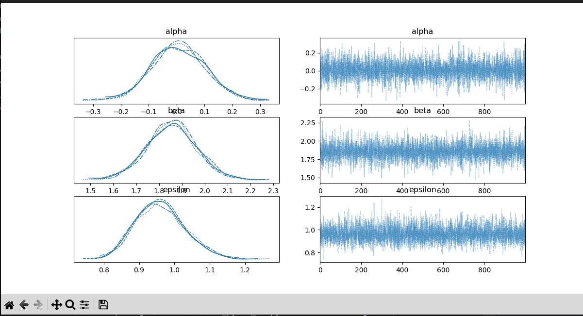
pm.traceplot(trace)
plt.show()

Code Breakdown:

1. Import Libraries:

   • pymc3provides tools for Bayesian modeling and probabilistic programming.

   • numpyused for numerical computations and array manipulation.

   • matplotlib.pyplotused for creating visualizations.

2. Simulate Data:

   • Creates a Gaussian random variable X with 100 values.

   • Generates a linear relationship y = 2 * X with added Gaussian noise.

3. Bayesian Linear Regression Model:

   • Defines a PyMC3 model with prior distributions for:

     • alpha: Intercept (mean 0, standard deviation 10).

     • beta: Slope (mean 0, standard deviation 10).

     • epsilon: Observation error (Half-Cauchy distribution with scale 5).

   • Declares the linear relationship mu = alpha + beta * X.

   • Observe the simulated data y.

4. Posterior Sampling:

   • Uses pm.sample to draw 1000 samples from the posterior distributions of the parameters.

   • Tune the sampler for 1000 iterations to improve convergence.

5. Plot Posterior Distributions:

   • Uses pm.traceplot to visualize the posterior distributions of alpha, beta, and epsilon.

   • Displays the plot using plt.show().

Example 2: Hierarchical Bayesian Model for Grouped Data

import pymc3 as pm
import numpy as np
import matplotlib.pyplot as plt

# Simulated grouped data (replace with your actual data)
np.random.seed(10)
num_groups = 5
group_sizes = np.random.randint(10, 20, size=num_groups)
grouped_data = []
for i in range(num_groups):
  true_alpha = np.random.rand() * 5
  group_data = true_alpha + np.random.randn(group_sizes[i])
  grouped_data.append(group_data)

# Define Hierarchical Bayesian Model
with pm.Model() as hierarchical_model:
  # Hyperparameters - Prior for group means
  mu_alpha = pm.Normal("mu_alpha", mu=0, sd=10)
  sigma_alpha = pm.HalfCauchy("sigma_alpha", 5)

  # Group-level random effects
  alpha = pm.Normal("alpha", mu=mu_alpha, sd=sigma_alpha, shape=len(grouped_data))

  # Likelihood for each group (assuming constant error term for simplicity)
  for i, data_group in enumerate(grouped_data):
    pm.Normal(f"y_obs_{i}", mu=alpha[i], sd=1, observed=data_group)

  # Sample from the posterior distribution
  trace_hierarchical = pm.sample(1000, tune=1000)

# Analyze and visualize posterior distributions
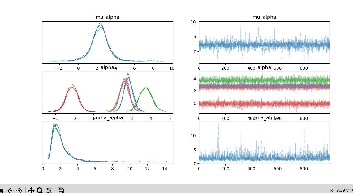
pm.traceplot(trace_hierarchical)
plt.show()

Explanation:

1. Import Libraries: Includes necessary libraries (pymc3, numpy, matplotlib).

2. Simulated Grouped Data: Creates example data with different group sizes for demonstration. Replace this with your actual data in groups.

3. Hierarchical Model:

   • Defines hyperparameters (mu_alpha, sigma_alpha) for the group-level random effects.

   • Creates a random effect (alpha) for each group based on the hyperparameters.

   • Defines the likelihood for each group's data assuming a normal distribution with mean from alpha and a fixed standard deviation (1 for simplicity).

4. Sampling: Performs MCMC sampling to obtain posterior distributions.

5. Visualization: Plots trace plots for the model parameters (mu_alpha, sigma_alpha, individual alpha for each group).

FAQs:

Q1: What advantages does the application of Bayesian Hierarchical Modeling offer?

A1: Bayesian Hierarchical Modeling accommodates intricate data structures, integrates past knowledge, and offers uncertainty estates.

Q2: Can real-world datasets be used with this method?

A2: Bayesian Hierarchical Modeling is indeed used in many fields, including biology, finance, and the social sciences.

Q3: How does MCMC function in Bayesian analysis?

A3: MCMC methods, like those implemented in PyMC3, enable sampling from complex posterior distributions, crucial in Bayesian analysis.

Q4: Are there alternatives to PyMC3 for Bayesian modeling?

A4: Yes, other libraries like Stan and JAGS are also popular choices for Bayesian modeling.

Conclusion:

In the machine learning toolbox, Bayesian Hierarchical Modeling is a potent tool that enables us to deal with structured data in an ethical manner and incorporate past knowledge. If we grasp the concepts behind Bayesian Hierarchical Modeling and the steps involved in developing one, we can utilize this tool to create machine learning models that are more dependable and comprehensible.